Mommy Vely

Merek Eyeliner Cair Terfavorit, Wajib Coba!

Eyeliner! Item make up yang satu ini ibarat penyelamat bagi mereka yang ingin mengoreksi bentuk mata agar terlihat lebih cantik dan menawan, sebab eyeliner mampu memberikan kesan mata yang tegas dan lebih hidup. Eyeliner sendiri terdiri dari beberapa jenis, mulai dari yang berbentuk cair, gel, juga pensil dan spidol. Bagi pemula, yang paling mudah digunakan adalah jenis pensil, spidol dan cair. Jenis cair sangat digemari karena mampu membuat eyeliner dengan bentuk yang rapi dan warna yang tegas. Bagi kamu yang ingin menggunakan eyeliner cair, berikut merek eyeliner cair rekomendasi dengan harga terjangkau namun kualitas terjamin.

Wardah Staylast Waterproof Liquid Eyeliner

Bila kamu seorang muslimah dan membutuhkan eyeliner yang halal dan berkualitas, kamu bisa mencoba Wardah Staylast Waterproof Liquid Eyeliner. Ini adalah eyeliner dari brand lokal yakni Wardah yang sudah dijamin halal. Produk ini akan memberikan finishing yang tampak glossy. Sementara itu, daya tahan yang ditawarkan eyeliner ini juga cukup bagus. Wardah Staylast Waterproof Liquid Eyeliner merupakan eyeliner yang tahan terhadap air, baik itu keringat maupun air mata, jadi aman untuk digunakan seharian tanpa takut luntur.

Viva Perfect Shape Liquid Eye Liner
Brand legendaris Viva merilis sebuah merk eyeliner cair yang bagus dan murah, yakni Perfect Shape Liquid Eye Liner. Produk ini berfungsi untuk membingkai mata dengan akurasi dan hasil ketajaman yang tinggi. Ada kuas aplikator yang nyaman untuk mengaplikasikan eyeliner di sekitar kelopak mata. Viva Perfect Shape Liquid Eye Liner ini memiliki kelebihan lebih cepat kering sehingga kegiatan merias mata bisa dilakukan secara lebih cepat. Eyeliner ini memiliki daya tahan selama 6 jam. Meskipun murah meriah, eyeliner cair dari Viva ini bersifat waterproof, yang artinya tahan air sehingga tidak mudah luntur begitu saja.

Revlon Colorstay Skinny Liquid Liner
Ini adalah salah satu merk eyeliner cair yang berkualitas bagus. Kuas eyeliner Revlon tergolong tebal, tetapi runcing di bagian ujung. Karakter kuas seperti ini akan membantumu untuk menggambar garis di tepi mata secara lebih rapi dan presisi. Revlon Colorstay Skinny Liquid Liner adalah eyeliner yang dapat kering secara cepat. Daya tahan eyeliner ini hingga 8 jam pemakaian. Ada dua pilihan warna yang tersedia, yaitu warna coklat dan hitam.

Pixy Perfect Eyeliner
Rekomendasi eyeliner cair terakhir datang dari merek Pixy. Bagi kamu yang kurang menyukai hasil akhir eyeliner yang matte, kamu bisa memilih eyeliner dari Pixy yang memiliki hasil akhir glossy nan cantik. Merek eyeliner cair yang bagus ini dirancang untuk menghasilkan warna hitam yang glossy dan juga pekat. Eyeliner Pixy ini juga bersifat waterproof sehingga tidak gampang luntur saat terkena air.

Itu dia beberapa merek eyeliner terfavorit yang digemari oleh banyak wanita Indonesia karena kualitasnya yang mumpuni dan didukung oleh harga yang sangat terjangkau. Eyeliner cair dari brand manakah yang menjadi pilihanmu?

Mobil LCGC Terbaik Daihatsu Ayla

Bukan rahasia lagi jika zaman ini harga mobil banyak yang sudah murah dan terjangkau. Hal ini sangat terlihat dari banyaknya mobil yang lalu lalang di jalanan. Kamu bisa memperhatikan bahwa kebanyakan yang punya mobil bukanlah orang yang punya harta banyak. Namun, kebanyakan mereka adalah kaum menengah. Sebenarnya mudah sekali untuk membedakan mana orang yang kaya beneran dengan menengah, bisa dilihat dari jenis mobil yang dia pakai. Jika dia menggunakan mobil LCGC yang tergolong murah, maka bisa dipastikan dia adalah orang yang ekonominya menengah. Namun, jika dia menggunakan mobil yang harganya di atas 500 juta, bisa dipastikan dia benar-benar orang yang kaya.

Tidak masalah kamu menjadi orang yang menengah atau orang kaya sekalipun, hal yang terpenting dari hidup ini sebenarnya adalah asal kamu bisa menikmati dan mensyukuri apa yang ada. Dengan mobil murah LCGC saja saya rasa sudah cukup membuatmu harus bersyukur jika dibandingkan orang yang ekonominya di bawah dirimu.

Terlepas dari masalah level ekonomi, mobil LCGC murah memang banyak diburu orang-orang saat ini. Pasalnya, terkadang seseorang sengaja membeli mobil yang murah untuk digunakan sebagai usaha rental mobil. Tentu saja hal ini sangat menguntungkan karena jika rental tidak laku pun dan ingin menjual mobil tersebut lagi ke pasaran, harganya juga tidak jatuh banyak seperti mobil premium lainnya. Selain itu, resiko menyewakan mobil dengan mobil LCGC juga lebih rendah.

Itu jika digunakan untuk rental mobil. Jika digunakan untuk kebutuhan pribadi, mobil LCGC juga sangat diminati. Yang pertama jelas karena harganya murah. Yang kedua, jelas dari sisi penggunaan bahan bakarnya yang hemat. Apalagi biasanya mobil ini digunakan untuk kerja yang notabene dilakukan tiap hari. Maka mencari mobil yang hemat bahan bakar sangat dicari.

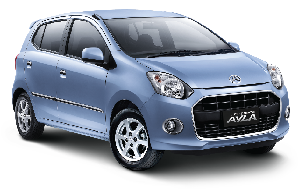
Salah satu mobil LCGC terbaik 2017 saat ini adalah mobil LCGC Daihatsu Ayla. Mobil LCGC ini meskipun murah, namun sudah dilengkapi dengan berbagai fitur dan kelebihan yang membuatmu puas. Daihatsu Ayla ini sudah dilengkapi dengan New Engine yang lebih powerful yaitu 1200 cc Dual VVT-i. Selain itu, Daihatsu Ayla ini juga menambah berbagai fitur keamanan, seperti: Dual SRS Airbag, Back Sonar, Side Impact Beam, Immobilizer & Alarm Integrated Key, Rear Stabilizer, Pedal Clutch Anti Back Up, dan fitur keamanan lainnya.

Bagaimana? Apakah kamu sekarang mulai tertarik dengan mobil murah Daihatsu Ayla ini?

4 Hal yang Perlu Diperhatikan Sebelum Membeli Apartemen

Terbatasnya lahan di kota-kota besar memang membuat harga jual rumah menjadi begitu mahal. Sehingga banyak orang yang kesulitan untuk mendapatkan tempat tinggal yang layak. Belum lagi tempat tinggal yang letaknya strategis dan nyaman memang terkesan diperuntukan untuk kalangan berduit. Salah satu kota yang menjadi kota terpadat di Indonesia yaitu Jakarta, memang terkenal dengan padatnya dan mahalnya harga properti di sana. Tapi bukan hal yang mustahil bagi kamu untuk tetap memiliki tempat tinggal yang nyaman dan aman di Jakarta.

Banyaknya dibagun apartemen di Jakarta Barat memang menjadi salah satu solusi untuk mengatasi kekurangannya tempat tinggal yang layak bagi para penduduk. Dengan adanya apartemen maka akan menghemat banyak lahan. Bagi kamu yang berminat untuk tinggal di apartemen di Jakarta Barat, berikut ini adalah tips sebelum membeli apartemen.

Cari Tahu Siapa Developernya

Kualitas apartemen yang akan kamu tinggal sangat berpengaruh dari siapa developer yang menggarap apartemen tersebut. Sehingga hal pertama yang harus kamu cari tahu sebelum membeli sebuah apartemen adalah siapa developernya. Jika developer tersebut memang memiliki reputasi bagus, maka kamu bisa mempertimbangkan untuk membeli apartemen tersebut.

Tanyakan Fasilitas yang Disediakan

Apartemen memang dirancang sebagai tempat tinggal yang ideal bagi penghuninya. Tak heran jika banyak apartemen yang memanjakan para penghuni dengan menyediakan berbagai fasilitas menarik. Tapi tidak semua orang membutuhkan fasilitas yang sama, sehingga sebelum kamu membeli apartemen, tentukan terlebih dahulu, fasilitas apa yang dibutuhkan. Jika kamu seorang yang single tentu saja tidak penting fasilitas taman bermain anak bukan? Jadi ada atau pun tidak fasilitas tersebut tidak berpengaruh pada pilihan kamu.

Perhitungkan Biaya Maintenance

Sama halnya dengan tinggal dipemukiman biasa, apartemen juga memiliki biaya bulanan yang harus dibayarkan. Kamu harus cermat mengenai biaya maintenace ini. Jangan sampai biaya dan layanan yang diberikan tidak sesuai.

Membeli Apartemen Lebih Awal

Jika kamu sudah menemukan apartemen yang sesuai dengan kebutuhan kamu, sekarang saatnya membeli apartemen yang kamu incar. Agar kamu bisa mendapatkan apartemen dengan harga yang lebih murah, kamu dapat melakukan pembelian apartemen lebih awal dari launching apartemen tersebut. Tapi tentu ini hanya berlaku jika apartemen yang akan kamu beli masih dalam tahap pembangunan. Dan memang sebisa mungkin carilah apartemen yang masih dalam tahap pembangunan sehingga kamu dapat mendapatkan harga yang lebih murah.

Kenapa Tinggal di Apartemen?

Terbatasnya lahan untuk tempat tinggal di kota-kota besar memang menjadi salah satu pemicu melambungnya harga jual rumah. Tidak heran jika rumah ukuran kecil dengan kondisi yang kurang layak dapat dibandrol yang cukup mahal. Belum lagi tempat-tempat tersebut juga belum tentu memiliki tempat yang strategis, atau pun aman untuk ditempati.

Selain dalam bentuk rumah, kamu juga memiliki pilihan hunian dalam bentuk apartemen. Memang mungkin apartemen berbeda dengan rumah. Tapi tentu saja memiliki banyak keuntungan jika dibandingkan dengan rumah biasa. Berikut adalah keuntungan jika kamu tinggal di apartemen.

Terletak di Area yang Strategis

Kebanyakan apartemen memang sengaja dibangun di tempat yang berdekatan dengan berbagai spot penting seperti gedung perkantoran, rumah sakit, sekolah, pusat berbelanjaan atau mall dan beberapa spot penting lainnya. Hal ini tentu saja memudahkan bagi para penghuni apartemen untuk dapat mencapai tempat-tempat penting tersebut tanpa harus menempuh waktu yang terlalu lama. Berbeda jika kamu tinggal di tempat yang jauh dari pusat kota. Maka kamu harus menempuh jarak yang cukup jauh, belum lagi harus terjebak macet di jalanan.

Fasilitas Tersedia di Area Apartemen

Berbeda dengan tinggal di pemukiman biasa, tinggal di apartemen kamu dapat menemukan banyak fasilitas yang tersedia dalam area apartemen. Sehingga jika kamu malas untuk keluar dari area apartemen kamu tinggal memanfaatkan fasilitas dari apartemen tersebut. Belum lagi biasanya ada juga layanan pesan antar untuk memenuhi kebutuhan kamu.

Keamanan Terjamin

Area apartemen bukanlah area yang dapat dimasukin sembarangan orang. Sehingga kemungkinan untuk dimasuki oleh orang asing sangat sedikit. Belum lagi dilengkapi dengan kamera CCTV dan juga petugas keamanan yang siaga selama dua puluh empat jam. Kamu tidak perlu khawatir lagi untuk meninggalkan apartemen dalam keadaan kosong.

Apartemen memang memiliki kesan tempat tinggal yang kecil. Tapi jika kamu membeli apartemen di jakarta Selatan Casa Grande Residence, kamu dapat memilih luas apartemen sesuai dengan kebutuhan kamu. Tersedia mulai dari apartemen yang memiliki satu kamar hingga empat kamar.

Beberapa keuntungan di atas dapat menjadi pertimbangan kamu saat memilih hunian yang nyaman untuk kamu maupun keluarga. Ingat selalu untuk memilih apartemen yang sesuai dengan kebutuhan kamu. Perhatikan fasilitas yang disediakan dan juga biaya maintenace yang dikenakan tiap bulannya. Juga pertimbangkan letak apartemen dengan tempat-tempat yang nantinya akan menjadi spot penting untuk kamu.

Keunggulan Data Center Lintasarta

Sudah bukan jamannya lagi menyimpan dokumen dalam bentuk kertas atau buku-buku. Di era digital ini, hampir kebanyakan dokumen penting berbentuk data digital. Sehingga dalam penyimpanannya pun memerlukan perangkat IT yang aman untuk menyimpan data. Banyak sekali cara menyimpan data penting pada perusahaan. Salah satunya adalah dengan menyimpan data tersebut pada perusahaan yang menyediakan layanan data center.

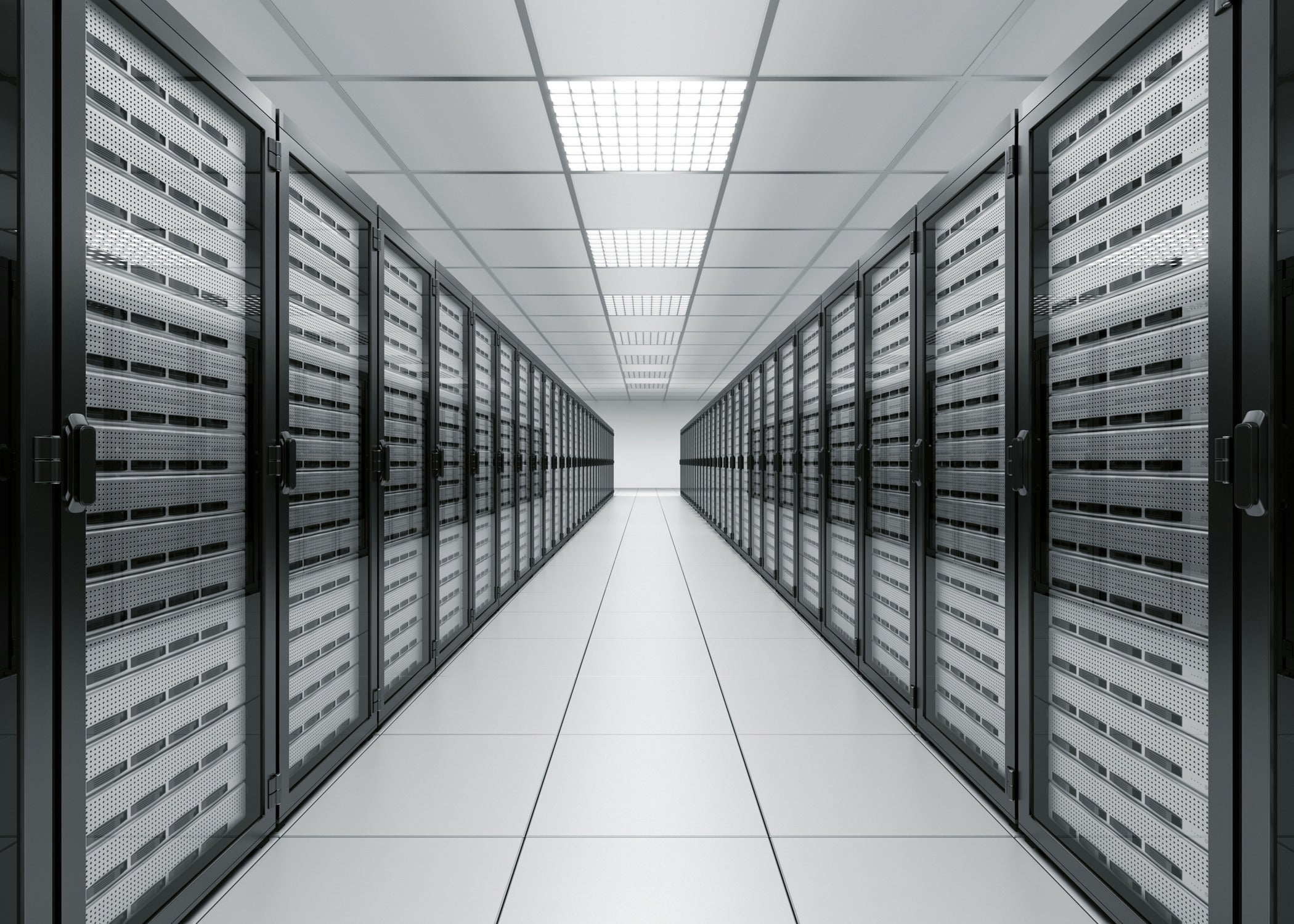
Banyak sekali penyedia data center membuat kamu harus berhati-hati dalam memilih data center yang handal untuk penyimpanan data penting perusahaan. Salah satu data center Indonesia yang dapat kamu andalkan adalah data center Lintasarta. Data center Lintasarta memiliki beberapa keunggulan berikut.

Disaster Recovery Center (DRC)

DRC atau Disaster Recovery Center adalah layanan yang menjamin data para pengguna agar tetap aman jika terjadi bencana. Sehingga kamu dapat tetap menjalankan bisnis tanpa harus terganggu dengan adanya bencana. Layanan Disaster Recovery Center ini berstandar internasional yang dapat kamu akses melalui jaringan dengan ketersediaan tinggi. Dan juga dikelola dan dipantau ketat oleh teknisi yang memiliki pengalaman dan keahlian di bidangnya.

Memiliki Lokasi yang Strategis dan Standar Keamanan yang Terjamin

Lokasi data center Lintasarta terdapat di tiga tempat. Yaitu, Jakarta, Bandung dan Jatiluhur. Setiap data center tersebut telah didukung dengan power supply yang stabil. Dan memiliki perlindungan pada bebagai kondisi seperti kebakaran. Dilengkapi juga dengan pengamanan berupa CCTV dan petugas keamanan yang handal.

Infrastruktur data center tersebut juga dilengkapi dengan ruangan pendingin, sehingga dapat mempertahankan suhu di dalam ruang agar tetap stabil. Dilengkapi juga dengan pengukur aliran udara dan tingkat kelembapannya yang terjagar. Dan semuanya berorprasi selama dua puluh empat jam.

Telah Tersertifikasi

Data center Lintasarta adalah data center yang telah memiliki pengalaman sebagai penyedia jasa komunikasi data selama lebih dari dua puluh tujuh tahun. Sehingga tidak heran jika data center Lintasarta berkualitas. Dilengkapi dengan SDM yang kompeten dan bersertifikasi CDCP (Certified Data Center Proferssional), CCIP (Cisco Certified Internetwork Professional), CCSP (Cisco Certified Security Professional) dan Certified Ethical Hacker).

Selain SDM yang tersertifikasi dan profesional pada bidangnya, kualitas layanan data center Lintasarta telah diaku dengan mendapatkannya sertifikasi ISO 9001:2008 Quality Management Systems, Sertifikasi ISO 27001:2005 Information Security Management Systems dan OHSAS 18001: 2007 Occupational Health and Safety Management System.

Jadi tunggu apa lagi, kamu bisa mempercayakan data penting pada bisnis kamu untuk disimpan di data center Lintasarta.